Smoking and Drinking Prediction
This data mining project course is centered on analyzing a Smoking and Drinking Dataset with body signals, which provides critical insights into patterns and factors contributing to drinking or smoking. The dataset serves as the foundation for exploring various data mining techniques and predictive modeling approaches. More detailed information about the dataset, including its structure, attributes, and data sources, can be found in the DATASET section of this page.

Team
Dataset
Aug 16, 2024
Description
This dataset, sourced from Kaggle, has been obtained from the National Health Insurance Service in Korea, with all personal and sensitive information removed. The dataset aims to facilitate the classification of individuals as smokers or drinkers. Here's a small sample:
| Index | Sex | Age | Height | Weight | Waistline | Sight Left | Sight Right | Hear Left | Hear Right | SBP | DBP | BLDS | Total Cholesterol | HDL Cholesterol | LDL Cholesterol | Triglyceride | Hemoglobin | Urine Protein | Serum Creatinine | SGOT AST | SGOT ALT | Gamma GTP | Smoking Status | Drinking Status |
|---|---|---|---|---|---|---|---|---|---|---|---|---|---|---|---|---|---|---|---|---|---|---|---|---|
| 0 | Male | 35 | 170 | 75 | 90.0 | 1.0 | 1.0 | 1.0 | 1.0 | 120.0 | 80.0 | 99.0 | 193.0 | 48.0 | 126.0 | 92.0 | 17.1 | 1.0 | 1.0 | 21.0 | 35.0 | 40.0 | 1.0 | Y |
| 1 | Male | 30 | 180 | 80 | 89.0 | 0.9 | 1.2 | 1.0 | 1.0 | 130.0 | 82.0 | 106.0 | 228.0 | 55.0 | 148.0 | 121.0 | 15.8 | 1.0 | 0.9 | 20.0 | 36.0 | 27.0 | 3.0 | N |
| 2 | Male | 40 | 165 | 75 | 91.0 | 1.2 | 1.5 | 1.0 | 1.0 | 120.0 | 70.0 | 98.0 | 136.0 | 41.0 | 74.0 | 104.0 | 15.8 | 1.0 | 0.9 | 47.0 | 32.0 | 68.0 | 1.0 | N |
| 3 | Male | 50 | 175 | 80 | 91.0 | 1.5 | 1.2 | 1.0 | 1.0 | 145.0 | 87.0 | 95.0 | 201.0 | 76.0 | 104.0 | 106.0 | 17.6 | 1.0 | 1.1 | 29.0 | 34.0 | 18.0 | 1.0 | N |
| 4 | Male | 50 | 165 | 60 | 80.0 | 1.0 | 1.2 | 1.0 | 1.0 | 138.0 | 82.0 | 101.0 | 199.0 | 61.0 | 117.0 | 104.0 | 13.8 | 1.0 | 0.8 | 19.0 | 12.0 | 25.0 | 1.0 | N |
This dataset has been sourced from Kaggle. For detailed information about the measures used in each column, please refer to the source.
Description of variables
| Index | Variable | Description |
|---|---|---|
| 1 | Sex | Indicates the individual's gender, which can be male or female. |
| 2 | Age | The individual's age, rounded to the nearest 5 years. |
| 3 | Height | The individual's height, rounded to the nearest 5 cm. |
| 4 | Weight | The individual's weight, measured in kilograms. |
| 5 | Sight_left | Visual acuity of the left eye, assessed as normal or abnormal. |
| 6 | Sight_right | Visual acuity of the right eye, assessed as normal or abnormal. |
| 7 | Hear_left | Hearing status of the left ear, classified as normal (1) or abnormal (2). |
| 8 | Hear_right | Hearing status of the right ear, classified as normal (1) or abnormal (2). |
| 9 | SBP (Systolic Blood Pressure) | The systolic blood pressure measurement, in mmHg. |
| 10 | DBP (Diastolic Blood Pressure) | The diastolic blood pressure measurement, in mmHg. |
| 11 | BLDS (Fasting Blood Glucose) | Blood glucose level after fasting, measured in mg/dL. |
| 12 | Tot_chole (Total Cholesterol) | Total cholesterol level in the blood, measured in mg/dL. |
| 13 | HDL_chole (HDL Cholesterol) | High-density lipoprotein cholesterol level in the blood, measured in mg/dL. |
| 14 | LDL_chole (LDL Cholesterol) | Low-density lipoprotein cholesterol level in the blood, measured in mg/dL. |
| 15 | Triglyceride | Triglyceride level in the blood, measured in mg/dL. |
| 16 | Hemoglobin | Hemoglobin concentration in the blood, measured in g/dL. |
| 17 | Urine_protein | Protein level in urine, classified from absence (-) to significant presence (+4). |
| 18 | Serum_creatinine | Serum creatinine level, measured in mg/dL. |
| 19 | SGOT_AST (SGOT/AST) | Serum level of aspartate aminotransferase (SGOT/AST), measured in IU/L. |
| 20 | SGOT_ALT (SGOT/ALT) | Serum level of alanine aminotransferase (SGOT/ALT), measured in IU/L. |
| 21 | Gamma_GTP | Serum level of gamma-glutamyl transpeptidase (Gamma-GTP), measured in IU/L. |
| 22 | SMK_stat_type_cd (Smoking Status) | Classification of smoking status, which can be never smoked (1), used to smoke but quit (2), or currently smoking (3). |
| 23 | DRK_YN (Drinker or Not) | Indicates whether the individual consumes alcohol or not. |
Justification
When patients are diagnosed with a respiratory problem or another health condition, they often show reluctance to reveal information about their smoking or drinking habits, and how frequently they engage in these activities. This lack of information may be due to various reasons, such as fear of being judged or appearing irresponsible about their health. As a result, doctors may face difficulties in providing appropriate treatment. To address this issue, it is crucial to obtain accurate information about the patient's smoking and drinking status without relying solely on their self-reports. Therefore, based on research, it has been shown that this information can be predicted from various measurable bodily signals, such as blood pressure, cholesterol, urine proteins, and certain enzymes. Thus, the main objective of this project is to train a machine learning model to predict the patients' status, providing a response that allows for verifying whether they consume alcohol and if they smoke frequently.
Goals
- Perform an exploratory analysis with the data that will be used on a machine learning model.
- Using that model, predict whether a person consumes alcohol or smokes.
Relevance
The primary goal of this project is to analyze body signals and classify individuals based on their smoking and drinking habits. The dataset aligns perfectly with these objectives by providing key health metrics (e.g., blood pressure, cholesterol levels, and liver enzymes) alongside smoking and drinking status. These variables are essential for identifying potential health risks associated with these habits, enabling the development of predictive models and classifications.
Case studies
Classifying smoking urges via machine learning
This study explores the use of machine learning methods to predict high-urge states during a smoking cessation attempt. Three classification approaches (Bayes, discriminant analysis, and decision trees) were evaluated using data from over 300 participants. The results indicated that decision trees, based on feature selection, achieved the highest accuracy, with 86% classification precision. This highlights the potential of machine learning to enhance smoking cessation interventions through mobile technologies, optimizing healthcare resources and providing personalized real-time support.
Analizing influence of smoking and alcohol drinking behaviors on body type with deep learning, machine learning and data mining techniques
This study examines the use of deep learning, machine learning, and data mining approaches to analyze the body types and consumption patterns of alcohol and smoking among various individuals. Despite numerous studies in the literature highlighting the risks and dangers of smoking and excessive, long-term alcohol use, there are also studies that emphasize and cite the benefits of limited and moderate alcohol consumption. The analysis aims to provide insights to leaders and society in general by investigating behaviors that have been present for centuries across different individuals, groups, and societies.
Hypotheses Based on Health Metrics for Predicting Smoking and Drinking Behaviors
Cholesterol (HDL, LDL, and Triglycerides):
Smoking: Smoking affects lipid profiles, with variations observed between adults and adolescents. In adult smokers, studies show higher levels of total cholesterol, LDL, VLDL, and triglycerides, and lower levels of HDL and apolipoprotein A. Adolescent smokers, however, often have lower levels of total cholesterol and HDL compared to non-smokers. Gender differences are also noted, with male smokers exhibiting a higher LDL/HDL ratio and a more pronounced reduction in HDL, potentially due to hormonal changes during puberty.
Drinking: Alcohol consumption has mixed effects on cholesterol and triglycerides. Moderate alcohol intake tends to increase HDL ("good" cholesterol), which benefits heart health. However, excessive alcohol consumption can raise LDL ("bad" cholesterol) levels, contributing to plaque buildup in arteries and increasing cardiovascular disease risk. Excessive drinking is also linked to elevated triglyceride levels, exacerbating cardiovascular risks.
Blood Pressure (SBP and DBP):
Smoking: Nicotine in cigarettes can elevate both systolic and diastolic blood pressure due to its vasoconstrictive effects, causing the heart to pump harder.
Drinking: Alcohol consumption is associated with increased systolic and diastolic blood pressure. This effect is more pronounced in individuals over 40 years old, while the relationship is less clear in younger individuals. Some older non-drinkers may have slightly higher blood pressure compared to moderate drinkers, possibly due to factors like obesity. Generally, reducing alcohol intake can help prevent hypertension.
Blood Glucose (BLDS):
Smoking: Smokers may have higher fasting blood glucose levels due to smoking's impact on insulin sensitivity, increasing the risk of type 2 diabetes.
Drinking: Chronic alcohol consumption can disrupt glucose regulation, potentially increasing or decreasing blood glucose levels depending on liver function.
Liver Enzymes (SGOT/AST, SGPT/ALT, Gamma-GTP):
Drinking: Excessive alcohol consumption is linked to elevated levels of liver enzymes such as Gamma-GTP, AST, and ALT, indicating liver damage or fatty liver, which are common in chronic drinkers.
Serum Creatinine:
Drinking: Alcohol can affect kidney function, which may be reflected in abnormal serum creatinine levels, especially with prolonged excessive drinking.
Improving Patient Care through Predictive Modeling:
To enhance patient diagnosis and treatment, it is crucial to use objective and precise data to predict behaviors such as smoking and drinking. By developing a model that predicts these behaviors based on health metrics like sex, age, height, weight, blood pressure, and cholesterol levels, healthcare providers can offer more personalized interventions. An effective model could identify individuals at risk of smoking or drinking based on their health characteristics, enabling tailored treatment plans. Additionally, the model could facilitate early intervention strategies by identifying risk patterns before they become serious, promoting more effective prevention and better health management.
References
- Bondía, J. P., Abaitua, F. R., López, R. E., Martínez, J. I., Mazón, H. F., Izurzu, Y. A., & Elízaga, I. V. (1997). Distribución de las variables lipídicas en adolescentes fumadores. An Esp Pediatr, 46, 245-251.
- Nasiff-Hadad, A., Gira, P., & Bruckert, E. (1997). Efectos del alcohol sobre las lipoproteínas. Revista Cubana de Medicina, 36(1), 51-60.
- Hernádez, J. P., Zanón, E. B., Rodríguez, F. S., Fácila, L., Gil, R. R., Díaz, P., & Mercé, S. Índice de Rigidez Arterial (SIDVP) y Velocidad de Onda de Pulso (baPWV) como estimadores de la Presión Arterial.
- Milon, H., Froment, A., Gaspard, P., Guidollet, J., & Ripoll, J. P. (1982). Alcohol consumption and blood pressure in a French epidemiological study. European heart journal, 3(suppl_C), 59-64.
- Valenzuela Magdaleno, A. Monitoreo continuo y automonitoreo de glucosa como seguimiento glucémico y autocuidado de pacientes con diabetes mellitus tipo 2.
Exploratory Data Analysis
Sep 13, 2024
Note: These are just conclusions. More detailed information can be found on the Google Colab jupyter notebook.
Exogenous repositories
These external sources could enhance the analysis in our project.
Worldwide Alcohol Consumption
This dataset is relevant to the project as it provides a global view of alcohol consumption, which will allow for the contextualization of drinking patterns in different regions of the world. This data could enrich the analysis by showing how cultural and geographical differences affect alcohol consumption habits, which could influence health biomarkers. Additionally, it will help identify how levels of alcohol consumption correlate with indicators such as cholesterol or blood pressure, providing an additional layer of analysis to the predictive model. This approach allows for adapting predictions to specific contexts based on the region, which could improve the accuracy and generalization of the model.
Smoking Signal of Body Classification
This dataset is relevant to the project as it shares the same objective as the project: predicting smoking habits based on body signals. This dataset not only provides a solid framework for building classification models but can also offer valuable insights into the most important variables for detecting smoking habits. The machine learning techniques applied in this analysis, such as SVM or Random Forest, can be reused or adjusted to optimize our own model, as they seek the same type of prediction based on biomarkers such as cholesterol, blood pressure, and other health indicators.
Data overview
The dataset consists of 991,346 observations and 24 variables.
Data Completeness
All variables are fully populated with no missing data.
Data Types:
- int64: 3 variables (e.g., age, height, weight)
- float64: 19 variables (e.g., waistline, cholesterol levels, blood pressure)
- object: 2 variables (e.g., sex, DRK_YN)
Next Steps:
- Data Quality: Check for consistency in categorical values.
- Outliers: Identify and handle any potential outliers.
We will proceed with a thorough analysis to ensure the data's reliability and readiness for further processing.
df_smk_drnk.info()Data columns (total 24 columns):
# Column Non-Null Count Dtype
--- ------ -------------- -----
0 sex 991346 non-null object
1 age 991346 non-null int64
2 height 991346 non-null int64
3 weight 991346 non-null int64
4 waistline 991346 non-null float64
5 sight_left 991346 non-null float64
6 sight_right 991346 non-null float64
7 hear_left 991346 non-null float64
8 hear_right 991346 non-null float64
9 SBP 991346 non-null float64
10 DBP 991346 non-null float64
11 BLDS 991346 non-null float64
12 tot_chole 991346 non-null float64
13 HDL_chole 991346 non-null float64
14 LDL_chole 991346 non-null float64
15 triglyceride 991346 non-null float64
16 hemoglobin 991346 non-null float64
17 urine_protein 991346 non-null float64
18 serum_creatinine 991346 non-null float64
19 SGOT_AST 991346 non-null float64
20 SGOT_ALT 991346 non-null float64
21 gamma_GTP 991346 non-null float64
22 SMK_stat_type_cd 991346 non-null float64
23 DRK_YN 991346 non-null object
dtypes: float64(19), int64(3), object(2)Converting Object Variables to Categorical Types
In this dataset, converting object variables to categorical types is a crucial step for efficient data handling and analysis. This conversion is essential for the following reasons:
- Memory Optimization: Converting object types to categorical reduces memory usage significantly.
- Ease of Analysis: Categorical data simplifies statistical analysis and modeling processes.
- Discrete Value Representation: Categorical variables represent discrete values, which is particularly important for:
- Group-Wise Operations: Facilitates operations and aggregations based on categories.
- Machine Learning Models: Enables the creation of dummy variables and improves model performance.
Variables such as sex, SMK_stat_type_cd, and DRK_YN are prime candidates for this conversion.
This can be done through the pd.Categorical() method. Taking sex as an example:
df_smk_drnk['sex'].unique()array(['Male', 'Female'], dtype=object)
# Map original values to new values
df_smk_drnk['sex'] = df_smk_drnk['sex'].map({'Male': 'M', 'Female': 'F'})
# Convert column to categorical type
df_smk_drnk['sex'] = pd.Categorical(df_smk_drnk['sex'], categories=['M', 'F'], ordered=True)
Doing the same to the rest of columns:
df_smk_drnk.info()Data columns (total 24 columns):
# Column Non-Null Count Dtype
--- ------ -------------- -----
0 sex 991346 non-null category
.
.
.
22 SMK_stat_type_cd 991346 non-null category
23 DRK_YN 991346 non-null category
dtypes: category(3), float64(18), int64(3)Data visualization
Analysis of categorical variables
Sex distribution
- M (Male): 526,415 individuals.
- F (Female): 464,931 individuals.
Interpretation: The dataset has a fairly balanced gender distribution, with a slightly higher number of males than females. This balance is beneficial for gender-specific analysis, as it minimizes the risk of gender bias in the results.

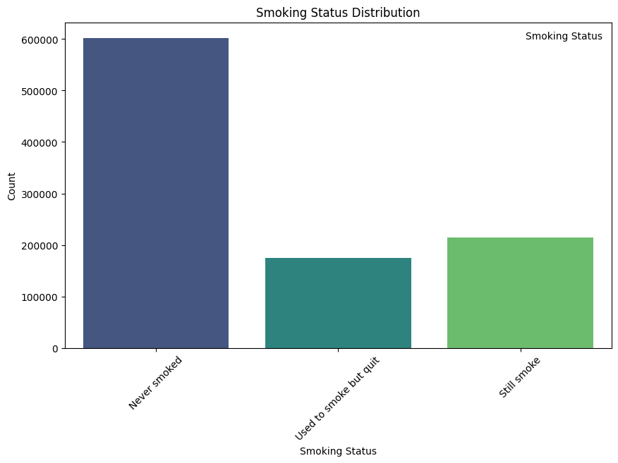
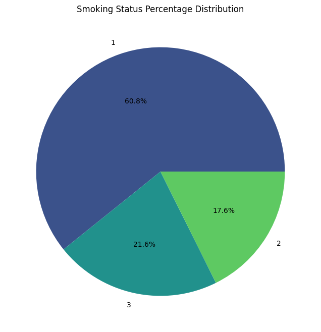
Smoking status (SMK_stat_type_cd)
- Never smoked: 602,441 individuals
- Still smoke: 213,954 individuals
- Used to smoke but quit 174,951 individuals
Interpretation: The majority of individuals (about 60.8%) in the dataset have never smoked. About 21.6% are current smokers, while 17.6% used to smoke but quit. This distribution allows for detailed analysis of smoking habits and their impact on health outcomes.
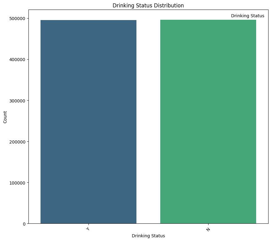
Drinking Status (DRK_YN)
- N (Non-drinkers): 495,858 individuals
- Y (Drinkers): 495,488 individuals
Interpretation: The dataset is almost perfectly balanced in terms of drinking status, with an almost equal split between drinkers and non-drinkers. This balance provides a solid foundation for comparative analysis between these two groups.
Age Distribution by Drinking Status
- Drinking appears to peak between the ages of 30 and 50, with a gradual decline starting around 50 years old.
- The number of non-drinkers increases with age, particularly after 60 years, potentially due to health concerns or lifestyle changes.
- Younger individuals (ages 20–30) show a noticeable presence of drinkers, but non-drinkers remain relatively close in count.
- Around ages 55–60, the proportion of non-drinkers surpasses that of drinkers. This shift suggests a critical age where drinking behavior declines substantially.

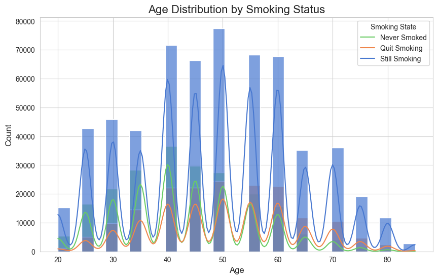
Age Distribution by Smoking Status
- The "Still Smoking" category (blue) has the highest density across all age groups, indicating that a significant portion of the population continues to smoke.
- The "Never Smoked" category (green) has a relatively consistent but lower density compared to "Still Smoking." This suggests that a smaller but steady group of individuals never pick up smoking across all ages.
- The "Quit Smoking" category (orange) appears to increase slightly with age, especially beyond 40 years. This may indicate that older individuals are more likely to quit smoking, possibly due to health concerns or lifestyle changes.
- Younger individuals (ages 20–30) show fewer instances of smoking (both active and quit), likely reflecting greater awareness or a shift in social norms discouraging smoking in recent years.
Pairplot of Key Body Signals by Drinking Status
- Both drinkers and non-drinkers have similar hemoglobin distributions, with minor differences visible in density. This suggests hemoglobin might not strongly differentiate drinkers from non-drinkers.
- Drinkers have a broader range and significantly higher values for gamma-GTP compared to non-drinkers. This confirms gamma-GTP as a potential key indicator for distinguishing drinkers due to its known association with liver stress from alcohol consumption.
- Most values for serum creatinine are concentrated at lower levels for both groups, with no significant visual separation between drinkers and non-drinkers.
RELATIONSHIPS:
- Hemoglobin vs. Gamma-GTP: No clear relationship is observed, but drinkers have more outliers for gamma-GTP at certain hemoglobin levels.
- Gamma-GTP vs. Serum Creatinine: There is no evident correlation, as serum creatinine values remain low regardless of gamma-GTP levels.

Pairplot of Key Body Signals by Smoking Status
- Never Smokers (1): Never-smokers generally have the highest hemoglobin levels, which is expected as they are not exposed to the harmful effects of smoking.
- Former Smokers (2): Former smokers seem to have intermediate hemoglobin levels between current smokers and never-smokers. This suggests that quitting smoking can lead to some recovery in hemoglobin levels over time.
- Smokers (3): Smokers tend to have slightly lower hemoglobin levels compared to never-smokers and former smokers. This could be due to various factors, including reduced oxygen-carrying capacity in the blood due to carbon monoxide exposure.
- Gamma-GTP: There's a clear difference in distribution. The "still smoke" group has a higher concentration of gamma-GTP compared to the other two groups. This could indicate potential liver damage or dysfunction associated with smoking.
- Serum Creatinine: The distribution is similar across all groups, suggesting no significant impact of smoking status on kidney function.
RELATIONSHIPS:
No clear relationship is visible between any of the variables
Data cleaning
Outliers
Outliers are data points that significantly differ from other observations in the dataset. They can be unusually high or low compared to the rest of the data and can arise due to variability in the data or errors in measurement.
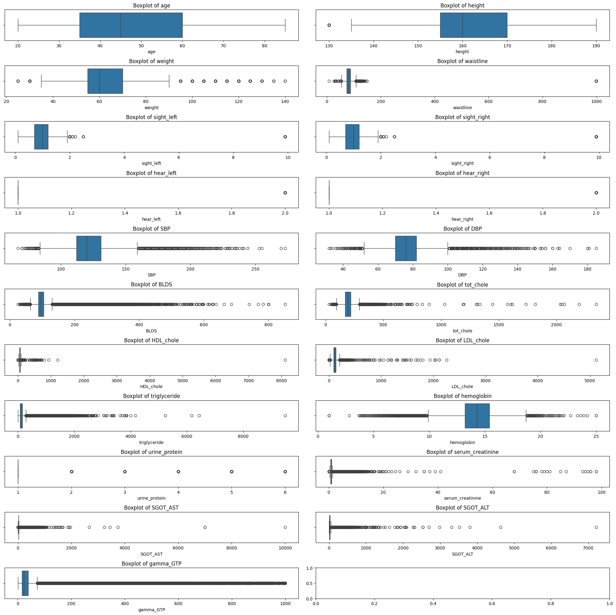
Outlier Detection Using Interquartile Range (IQR)
- Technique: The IQR method was used to detect outliers. It involves calculating the first quartile (Q1) and the third quartile (Q3) of the data for each numeric feature. The interquartile range (IQR) is then calculated as the difference between Q3 and Q1. Outliers are identified as data points that fall below Q1 - 1.5 * IQR or above Q3 + 1.5 * IQR.
- Reason: The IQR method is a robust technique that is less sensitive to extreme values than methods based on mean and standard deviation. It is commonly used for datasets that may have non-normal distributions, which is often the case in medical data.
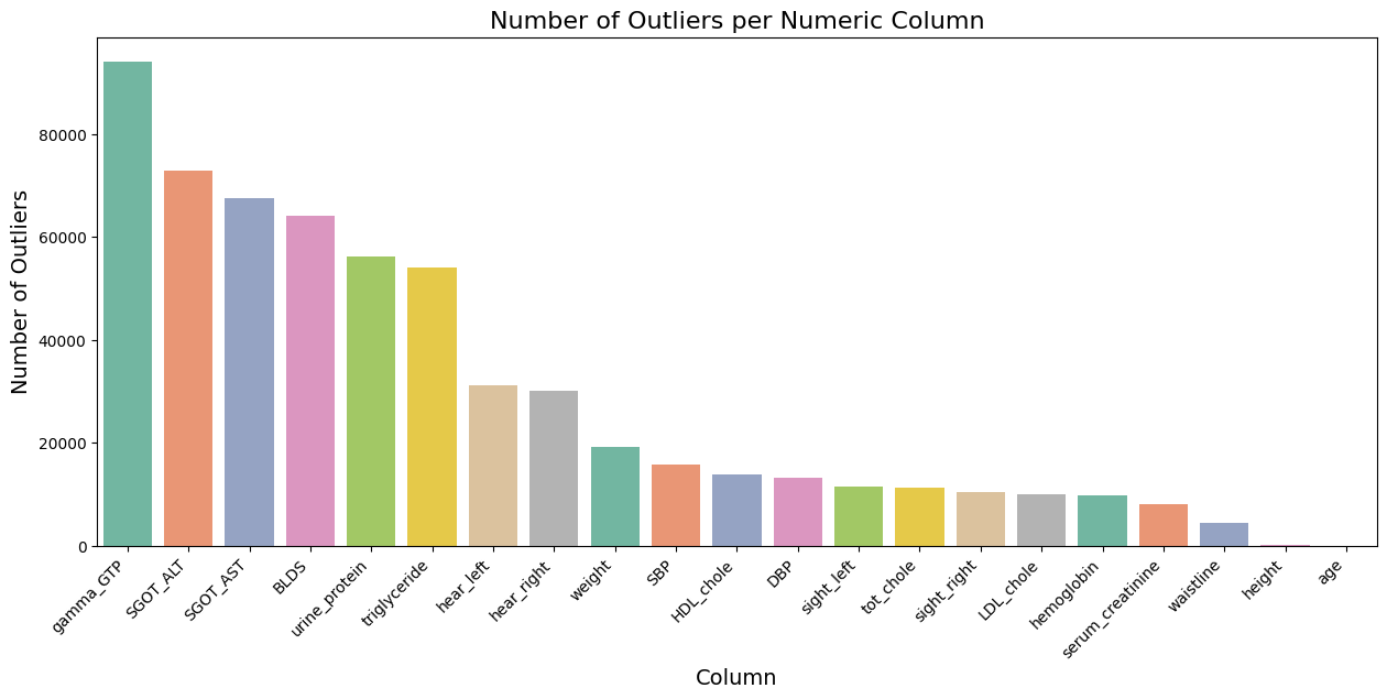
- Action: Identified outliers were visualized using boxplots, and their counts were plotted to determine the extent of the issue. Outliers were removed to create a cleaner dataset for further analysis.
# Select only numeric columns for outlier detection
numeric_cols = df_smk_drnk.select_dtypes(include=[np.number]).columns

# Calculate the IQR for each column
Q1 = df_smk_drnk[numeric_cols].quantile(0.25)
Q3 = df_smk_drnk[numeric_cols].quantile(0.75)
IQR = Q3 - Q1

# Define outliers using the IQR method
outliers = ((df_smk_drnk[numeric_cols] < (Q1 - 1.5 * IQR)) | (df_smk_drnk[numeric_cols] > (Q3 + 1.5 * IQR)))
Plotting:
Data imputation
There are no missing values in the dataset.
print((df_cleaned.isnull().sum() / len(df_cleaned)) * 100).
sex 0.0
age 0.0
height 0.0
weight 0.0
waistline 0.0
sight_left 0.0
sight_right 0.0
hear_left 0.0
hear_right 0.0
SBP 0.0
DBP 0.0
BLDS 0.0
tot_chole 0.0
HDL_chole 0.0
LDL_chole 0.0
triglyceride 0.0
hemoglobin 0.0
urine_protein 0.0
serum_creatinine 0.0
SGOT_AST 0.0
SGOT_ALT 0.0
gamma_GTP 0.0
SMK_stat_type_cd 0.0
DRK_YN 0.0
dtype: float64There were 14 duplicated rows.
num_duplicated = df_cleaned.duplicated().sum()
print(f'Number of duplicate rows: {num_duplicated}')
Number of duplicate rows: 14
After elimination:
df_cleaned.drop_duplicates(inplace=True)
num_duplicated = df_cleaned.duplicated().sum()
print(f'Number of duplicate rows: {num_duplicated}')
Number of duplicate rows: 0
Data Migration to Google BigQuery
Oct 18, 2024
Migration Plan
After completing the data cleaning process and obtaining a clean dataset, the migration of the data to BigQuery was carried out. Before performing the migration, the following steps were taken:
-
Transformation of Categorical Columns:
-
SMK_stat_type_cd: Converted to integer (int8).
-
sex and DRK_YN: Converted to text (string).
-
-
Encoding of Categorical Columns:
- A label encoder was applied to transform the sex column, where "Male" was converted to 1 and "Female" to 0. Similarly, the DRK_YN column was transformed, assigning the value 1 for "Y" and 0 for "N".
-
Verification of Numeric Column Formats:
- It was checked that the numeric columns were correctly formatted as int64 or float64.
-
Loading Strategy:
-
The
pandas_gbq.to_gbqfunction was used to perform the migration in a single operation, utilizing the optionif_exists='replace'to replace the table if it already existed. - The migration was carried out using credentials from a service account with write permissions in BigQuery.
-
The
Execution of the Migration Process
-
Environment Setup:
- Credentials were configured using the JSON file of the service account to establish the connection with BigQuery.
-
Data Upload:
-
The
pandas_gbq.to_gbq()function was employed to load the dataset from pandas to BigQuery.
-
The
-
Verification of the Load:
- Once the load was completed, the correct migration was verified through simple SQL queries in BigQuery.
Challenges Encountered and Solutions
-
403 Access Denied:
- Problem: The service account did not have the necessary permissions to create datasets.
- Solution: The roles BigQuery Data Editor and BigQuery Admin were assigned to the service account from the Google Cloud Console.
-
Incorrect Table Name Format:
- Problem: Initially, an incorrect table name format was used.
- Solution: The format was adjusted to
dataset.table, removing the project reference from the table name.
Model
Oct 18, 2024
For this task, the RandomForestClassifier model was selected due to its robustness and ability to handle a large number
of features effectively.
Training
Data Splitting
The dataset was split into training (70%) and test (30%) sets using train_test_split with stratification to maintain the balance of classes in both sets.
Model Training
- Training Data: The training data was used to fit the
RandomForestClassifier. - Feature Scaling: We applied
StandardScalerto ensure all features were on the same scale.
Computational Resources
The training was conducted on Google Colab, which provided ample CPU resources for model training.
Stratified 10-Fold Cross-Validation
To evaluate the model's performance effectively, we implemented Stratified 10-Fold Cross-Validation. This method was chosen specifically to maintain the class distribution across each fold, which is crucial when dealing with imbalanced datasets. By ensuring that each training and testing set reflects the overall class distribution, we can mitigate potential biases and improve the reliability of our model evaluation.
Here is an overview of the function:
def train_model(df, target_col, model_name):

    X = df.drop(columns=['SMK_stat_type_cd', 'DRK_YN'])  # Features (excluding target variables)
    y = df[target_col]  # Target (smoking or drinking)

    # Split data into training and test sets (70% training, 30% testing)
    X_train, X_test, y_train, y_test = train_test_split(X, y, test_size=0.3, random_state=42, stratify=y)

    # Feature scaling
    scaler = StandardScaler()
    X_train_scaled = scaler.fit_transform(X_train)
    X_test_scaled = scaler.transform(X_test)

    # Initialize RandomForestClassifier
    rf_model = RandomForestClassifier(random_state=42, n_estimators=100, max_depth=10, min_samples_split=5)

    # Train the model
    rf_model.fit(X_train_scaled, y_train)

    # Model Evaluation on the test set
    y_pred = rf_model.predict(X_test_scaled)

    # Performance metrics
    accuracy = accuracy_score(y_test, y_pred)
    precision = precision_score(y_test, y_pred, average='macro')
    recall = recall_score(y_test, y_pred, average='macro')
    f1 = f1_score(y_test, y_pred, average='macro')

    # Confusion matrix
    conf_matrix = confusion_matrix(y_test, y_pred)

    # Print formatted results
    print(f'# {model_name} Classification Results
')
    print(f'**Accuracy:** {accuracy:.3f}')
    print(f'**Precision:** {precision:.3f}')
    print(f'**Recall:** {recall:.3f}')
    print(f'**F1-Score:** {f1:.3f}
')

    print(f'## Classification Report:')
    print(classification_report(y_test, y_pred))

    # Cross-validation with StratifiedKFold
    cv = StratifiedKFold(n_splits=10, shuffle=True, random_state=42)
    cv_scores = cross_val_score(rf_model, X_train_scaled, y_train, cv=cv, scoring='accuracy')

    # Print cross-validation results
    print(f'## Cross-Validation Accuracy Scores: {cv_scores}')
    print(f'**Mean CV Accuracy:** {np.mean(cv_scores):.3f}
')

    # Return model, confusion matrix, test labels, and unscaled X_train for feature importance
    return rf_model, conf_matrix, y_test, X_train
Smoking Status
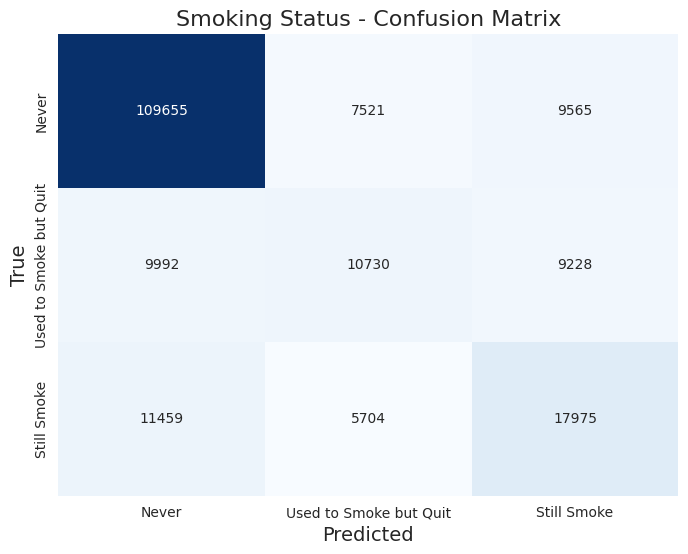
The classificacion report returned these results:
Accuracy: 0.721
Precision: 0.590
Recall: 0.579
F1-Score: 0.583
Classification Report:
| Label | Precision | Recall | F1-Score | Support |
|---|---|---|---|---|
| 1.0 (never) | 0.84 | 0.86 | 0.85 | 126,741 |
| 2.0 (used to smoke but quit) | 0.45 | 0.36 | 0.40 | 29,950 |
| 3.0 (still smoke) | 0.49 | 0.51 | 0.50 | 35,138 |
Cross-Validation Accuracy Scores:
0.72062109, 0.72017426, 0.72231903, 0.71899017, 0.7169571, 0.72115728, 0.71925827, 0.71624218, 0.71919124, 0.72097232
Mean CV Accuracy: 0.720
Here is the confusion matrix:

Drinking Status
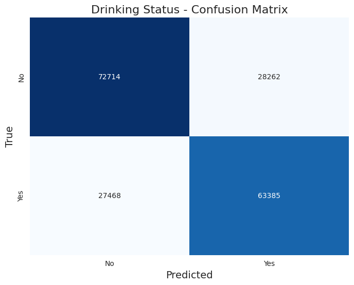
The classificacion report returned these results:
Accuracy: 0.709
Precision: 0.709
Recall: 0.709
F1-Score: 0.709
Classification Report:
| Label | Precision | Recall | F1-Score | Support |
|---|---|---|---|---|
| 0.0 (No) | 0.73 | 0.72 | 0.72 | 100,976 |
| 1.0 (Yes) | 0.69 | 0.70 | 0.69 | 90,853 |
Cross-Validation Accuracy Scores:
0.70828865, 0.70976318, 0.70989723, 0.70781948, 0.70958445, 0.70735031, 0.70504915, 0.70592046, 0.70607685, 0.70703099
Mean CV Accuracy: 0.708
Here is the confusion matrix:
Hyperparameter Tuning
We implemented hyperparameter tuning to optimize our model's performance by finding the best combination of hyperparameters, which helps improve accuracy, reduce overfitting, and ensure that the model generalizes well to unseen data.
def tuning(df, target_col, n_iter=20):
    """
    Train a Random Forest model with hyperparameter tuning using a subset of data.

    Parameters:
    -----------
    df : pandas.DataFrame
        Input dataframe containing features and target
    target_col : str
        Name of the target column
    n_iter : int, optional
        Number of parameter combinations to try in random search

    Returns:
    --------
    dict
        Dictionary containing the best parameters
    """

    # Separate features and target
    list_of_columns = df.columns.tolist()
    list_of_columns.remove(target_col)
    feature_cols = list_of_columns

    # Use a 30% sample of the df for tuning
    df_sample = df.sample(frac=0.4, random_state=42)

    X = df_sample[feature_cols]
    y = df_sample[target_col]

    # Split data for training the hyperparameter tuning model
    X_train, _, y_train, _ = train_test_split(X, y, test_size=0.3, random_state=42, stratify=y)

    # Parameter grid for Random Forest
    params = {
    'n_estimators': [100, 200, 300],
    'max_depth': [10, 20, 30, 40, None],
    'min_samples_split': [2, 5, 10],
    'min_samples_leaf': [1, 2, 4],
    'max_features': ['sqrt', 'log2', None],
    'bootstrap': [True, False],
    'class_weight': ['balanced', 'balanced_subsample', None]
}

    # Initialize Random Forest
    rf = RandomForestClassifier(random_state=42, n_jobs=-1)

    # Setup cross-validation
    skf = StratifiedKFold(n_splits=5, shuffle=True, random_state=42)

    # Initialize RandomizedSearchCV
    random_search = RandomizedSearchCV(
        estimator=rf,
        param_distributions=params,
        n_iter=n_iter,
        scoring='accuracy',  # Can adjust scoring if desired
        n_jobs=-1,
        cv=skf.split(X_train, y_train),
        verbose=1,
        random_state=42
    )

    # Start timing and fit
    print("Starting parameter search...")
    start_time = timer()
    random_search.fit(X_train, y_train)
    timer(start_time)

    # Return only the best parameters
    return {
        'best_params': random_search.best_params_
    }
Tuning both smoking and drinking:
Smoking status after hypertuning
best_params_smoking = tuning(df_smoking_important, target_col='SMK_stat_type_cd')Time taken: 0 hours 19 minutes and 23.08 seconds.
{'best_params': {'n_estimators': 300,
'min_samples_split': 5,
'min_samples_leaf': 4,
'max_features': 'log2',
'max_depth': 10,
'class_weight': None,
'bootstrap': True}}Using these parameters on the training we got these results:
Accuracy: 0.721
Precision: 0.591
Recall: 0.578
F1-Score: 0.583
Classification Report:
| Label | Precision | Recall | F1-Score | Support |
|---|---|---|---|---|
| 1.0 (never) | 0.84 | 0.87 | 0.85 | 126,741 |
| 2.0 (used to smoke but quit) | 0.45 | 0.36 | 0.40 | 29,950 |
| 3.0 (still smoke) | 0.49 | 0.51 | 0.50 | 35,138 |
Cross-Validation Accuracy Scores:
0.72004021, 0.7204647, 0.72287757, 0.71970509, 0.71785076, 0.72033065, 0.72010724, 0.71726988, 0.72015192, 0.72092763
Mean CV Accuracy: 0.720
Here is the confusion matrix:
There are features that are driving the Random Forest model's predictions:
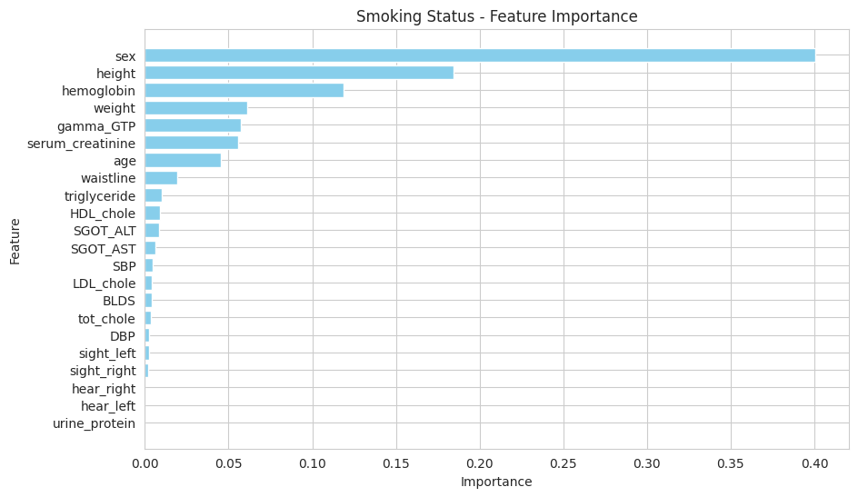
Feature Importance
The most important features identified for predicting smoking status are:
- Sex
- Height
- Hemoglobin
- Weight
- Gamma-GTP
- Serum Creatinine
- Age
These features play a significant role in the model's decision-making process, indicating that biological and demographic factors are crucial in assessing smoking status.
Insights and Discrepancies
The model achieved an overall accuracy of 72.1%, which is indicative of a decent performance in classifying smoking status. However, the precision and recall metrics reveal some important insights:
- Class Imbalance: The model performs significantly better for the first class (smoking status 1.0) with a precision of 0.84 and a recall of 0.86. This suggests that the model is effective in identifying non-smokers. However, the lower precision (0.45) and recall (0.36) for the second class (status 2.0) indicate that it struggles to accurately classify occasional smokers. The performance for the third class (status 3.0) is slightly better but still lacks robustness (precision: 0.49, recall: 0.51).
- F1-Score Analysis: The F1-scores highlight the trade-offs between precision and recall for different classes. The first class achieves an F1-score of 0.85, while the second and third classes only achieve 0.40 and 0.50, respectively. This suggests that while the model is reliable for the majority class, it is not performing well for the minority classes.
- Cross-Validation Consistency: The mean cross-validation accuracy of 72.0% corroborates the overall accuracy, indicating that the model's performance is consistent across different subsets of the data. However, the variability in the scores suggests there might be fluctuations in performance depending on the specific data split used.
In summary, while the smoking status classification model shows promise, particularly in identifying non-smokers, there are significant challenges in accurately classifying occasional and heavy smokers. Addressing class imbalance, perhaps through techniques like oversampling, undersampling, or model adjustments, could help improve the model's performance across all classes.
Drinking status after hypertuning
best_params_drinking = tuning(df_drinking_important, target_col='DRK_YN')Time taken: 0 hours 18 minutes and 35.05 seconds.
{'best_params': {'n_estimators': 300,
'min_samples_split': 5,
'min_samples_leaf': 4,
'max_features': 'log2',
'max_depth': None,
'class_weight': None,
'bootstrap': True}}Using these parameters on the training we got these results:
Accuracy: 0.716
Precision: 0.715
Recall: 0.715
F1-Score: 0.715
Classification Report:
| Label | Precision | Recall | F1-Score | Support |
|---|---|---|---|---|
| 0.0 (No) | 0.73 | 0.73 | 0.73 | 100,976 |
| 1.0 (Yes) | 0.70 | 0.70 | 0.70 | 90,853 |
Cross-Validation Accuracy Scores:
0.71423146, 0.71713584, 0.71456658, 0.71416443, 0.71525916, 0.71394102, 0.71251117, 0.71389634, 0.71134942, 0.71353247
Mean CV Accuracy: 0.714
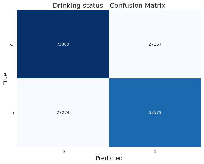
Here is the confusion matrix:
There are features that are driving the Random Forest model's predictions:
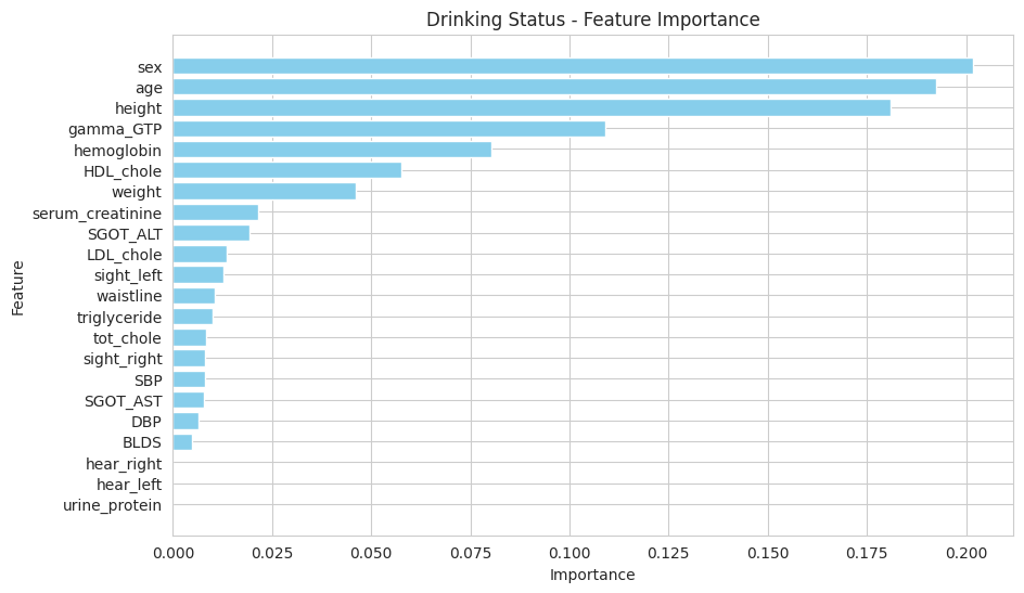
Feature Importance
The most important features identified for predicting drinking status are:
- Gamma-GTP
- Age
- Hemoglobin
- HDL Cholesterol
- Triglycerides
- Height
- LDL Cholesterol
These features play a significant role in the model's decision-making process, suggesting that biological and lifestyle factors are crucial in assessing drinking status.
Insights and Discrepancies
The model achieved an overall accuracy of 71.2%, indicating a solid performance in classifying drinking status. The metrics reveal several key insights:
- Balanced Performance: The precision, recall, and F1-scores are all approximately equal across both classes, reflecting a balanced performance between non-drinkers (0.0) and drinkers (1.0). Specifically, the model shows a precision of 0.72 and recall of 0.74 for non-drinkers, while for drinkers, the precision is 0.70 and recall is 0.69. This suggests that the model is fairly reliable for both categories.
- F1-Score Consistency: The F1-scores are also close to each other, with 0.73 for non-drinkers and 0.69 for drinkers. This consistency indicates that the model maintains a good balance between false positives and false negatives across both classes.
- Cross-Validation Results: The mean cross-validation accuracy of 71.0% aligns closely with the overall accuracy, suggesting that the model’s performance is stable across different subsets of the data. The slight fluctuations in individual cross-validation scores (ranging from 0.706 to 0.712) indicate a reliable but slightly sensitive model, potentially influenced by the distribution of classes in each fold.
- Class Support: The support for each class indicates that the dataset has a higher number of non-drinkers (100,976) compared to drinkers (90,853). This could suggest a potential class imbalance issue that may affect the model's performance in real-world applications, although the metrics do not currently indicate severe bias.
In conclusion, the drinking status classification model demonstrates solid performance, especially in distinguishing between non-drinkers and drinkers. However, continued monitoring and possibly addressing any latent class imbalance through data augmentation or model tuning could further enhance the model's robustness and predictive capability.
Dashboard
Nov 15, 2024